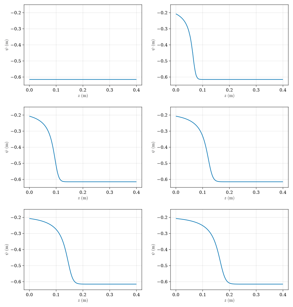
Celia et al. (1990) infiltration problem
This tutorial runs the one-dimensional Richards benchmark from the following paper:
Celia, M. A., Bouloutas, E. T., Zarba, R. L. (1990). A general mass-conservative numerical solution for the unsaturated flow equation. Water Resources Research, 26(7), 1483-1496. DOI: 10.1029/WR026i007p01483
First, we load the required packages.
using HydroTrixi
using SciMLBase
using Trixi
Solve the Richards problem
The setup below follows the elixir_richards_celia_1990.jl example, but we keep a saved time history so the same solution object can drive the animation step later in the tutorial.
asset_dir = docs_generated_dir("celia_1990")"/home/runner/work/HydroTrixi.jl/HydroTrixi.jl/docs/src/assets/generated/celia_1990"1. Load the benchmark definition
HydrologicProblemCelia1990 packages the Richards equation, water retention maps, boundary data, spatial domain, and time interval for the standard infiltration problem.
problem = HydrologicProblemCelia1990()┌──────────────────────────────────────────────────────────────────────────────────────────────────┐
│ HydrologicProblem │
│ ═════════════════ │
│ #spatial dimensions: ……………………………………… 1 │
│ equations: ………………………………………………………………… RichardsEquation1D │
│ initial condition: …………………………………………… initial_condition │
│ boundary conditions: ……………………………………… 2 │
│ │ negative x: ………………………………………………………… BoundaryConditionDirichlet │
│ │ positive x: ………………………………………………………… BoundaryConditionDirichlet │
│ domain: ………………………………………………………………………… ((0.0,), (0.4,)) │
│ time interval: ……………………………………………………… (0.0, 360.0) │
│ source terms: ………………………………………………………… nothing │
│ state to evolved: ……………………………………………… water_content │
│ evolved to state: ……………………………………………… pressure_head_from_water_content │
└──────────────────────────────────────────────────────────────────────────────────────────────────┘2. Build the mesh
The benchmark is one-dimensional, so a TreeMesh with five levels of initial refinement gives 32 cells before time integration begins.
mesh = TreeMesh(problem.domain...,
                initial_refinement_level = 5,
                n_cells_max = 30_000)
┌──────────────────────────────────────────────────────────────────────────────────────────────────┐
│ TreeMesh{1, Trixi.SerialTree{1, Float64}} │
│ ═════════════════════════════════════════ │
│ center: ………………………………………………………………………… [0.2] │
│ length: ………………………………………………………………………… 0.4 │
│ periodicity: …………………………………………………………… (false,) │
│ current #cells: …………………………………………………… 63 │
│ #leaf-cells: …………………………………………………………… 32 │
│ current capacity: ……………………………………………… 30000 │
└──────────────────────────────────────────────────────────────────────────────────────────────────┘3. Set up the spatial discretization
We use a polynomial degree of $N = 3$ together with the mixed implicit Richards semidiscretization SemidiscretizationImplicit, using a local DG (LDG) formulation for the parabolic solver.
solver = DGSEM(polydeg = 3)

semi = SemidiscretizationImplicit(mesh, problem, solver;
                                  solver_parabolic = ParabolicFormulationLocalDG())
┌──────────────────────────────────────────────────────────────────────────────────────────────────┐
│ SemidiscretizationImplicit │
│ ══════════════════════════ │
│ #spatial dimensions: ……………………………………… 1 │
│ mesh: ……………………………………………………………………………… TreeMesh{1, Trixi.SerialTree{1, Float64}} with length 63 │
│ equations: ………………………………………………………………… RichardsEquation1D │
│ initial condition: …………………………………………… initial_condition │
│ boundary conditions: ……………………………………… 2 │
│ │ negative x: ………………………………………………………… BoundaryConditionDirichlet │
│ │ positive x: ………………………………………………………… BoundaryConditionDirichlet │
│ source terms: ………………………………………………………… nothing │
│ solver: ………………………………………………………………………… DG │
│ parabolic solver: ……………………………………………… ParabolicFormulationLocalDG │
│ temporal operator: …………………………………………… TemporalOperatorConstitutive │
│ state to evolved: ……………………………………………… water_content │
│ evolved to state: ……………………………………………… pressure_head_from_water_content │
│ total #DOFs per field: ………………………………… 128 │
└──────────────────────────────────────────────────────────────────────────────────────────────────┘4. Solve and keep a time history
The Richards problem is stiff, so default_algorithm selects the Rodas5P Rosenbrock method from the SciML ecosystem. The time step is adaptive, with an initial step size of $\Delta t = 1.0 \times 10^{-2}$ seconds. We specify saveat = 0.0:6.0:360.0 to save a solution every six seconds, which will be used to create an animation in the next tutorial section. The adaptive = true keyword below controls time adaptivity only; see examples/elixir_richards_celia_1990_amr.jl for mesh adaptivity based on water content.
ode = semidiscretize(semi, problem.tspan)

sol = solve(ode,
            default_algorithm(semi);
            dt = 1.0e-2,
            adaptive = true,
            saveat = 0.0:6.0:360.0,
            save_everystep = false,
            maxiters = typemax(Int))

println("Solved Richards problem to t = $(sol.t[end]) with $(length(sol.t)) saved states.")
Solved Richards problem to t = 360.0 with 61 saved states.
Plot the final pressure head profile
Now that the solve is complete, we load the optional plotting packages. HydroTrixi declares these packages as weak dependencies, so a fresh package environment may not have them installed yet. If using CairoMakie fails, install the plotting packages in the active environment before continuing:
using Pkg
Pkg.add(["CairoMakie", "LaTeXStrings"])
using CairoMakie
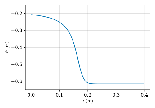
using LaTeXStringsThe mixed Richards formulation stores both evolved and state variables. The pressure head lives in the state block, so we plot component = 2 with plot_solution_1d. The output file is written into the docs asset directory prepared by the build.
plot_path = joinpath(asset_dir, "richards_celia_1990_pressure_head.png")

_ = plot_solution_1d(sol;
                     component = 2,
                     xlabel = L"$z$ (m)",
                     ylabel = L"$\psi$ (m)",
                     ylims = (-0.65, -0.15),
                     output_path = plot_path)

println("Saved final-time plot to $(plot_path)")
Saved final-time plot to /home/runner/work/HydroTrixi.jl/HydroTrixi.jl/docs/src/assets/generated/celia_1990/richards_celia_1990_pressure_head.png
Render the GIF animation
Because the solve already stored a time history, animate_solution_1d only needs to read the saved states and render them.
animation_path = joinpath(asset_dir, "richards_celia_1990_pressure_head.gif")

_ = animate_solution_1d(sol;
                        component = 2,
                        xlabel = L"$z$ (m)",
                        ylabel = L"$\psi$ (m)",
                        ylims = (-0.65, -0.15),
                        output_path = animation_path,
                        framerate = 20)

println("Saved animation to $(animation_path)")
Saved animation to /home/runner/work/HydroTrixi.jl/HydroTrixi.jl/docs/src/assets/generated/celia_1990/richards_celia_1990_pressure_head.gif